Why divide the sample variance by N-1?
Contents
Introduction
In this article, we will derive the well known formulas for calculating the mean and the variance of normally distributed data, in order to answer the question in the article’s title. However, for readers who are not interested in the ‘why’ of this question but only in the ‘when’, the answer is quite simple:
If you have to estimate both the mean and the variance of the data (which is typically the case), then divide by N-1, such that the variance is obtained as:
If, on the other hand, the mean of the true population is known such that only the variance needs to be estimated, then divide by N, such that the variance is obtained as:
Whereas the former is what you will typically need, an example of the latter would be the estimation of the spread of white Gaussian noise. Since the mean of white Gaussian noise is known to be zero, only the variance needs to be estimated in this case.
If data is normally distributed we can completely characterize it by its mean ![]() and its variance
and its variance ![]() . The variance is the square of the standard deviation
. The variance is the square of the standard deviation ![]() which represents the average deviation of each data point to the mean. In other words, the variance represents the spread of the data. For normally distributed data, 68.3% of the observations will have a value between
which represents the average deviation of each data point to the mean. In other words, the variance represents the spread of the data. For normally distributed data, 68.3% of the observations will have a value between ![]() and
and ![]() . This is illustrated by the following figure which shows a Gaussian density function with mean
. This is illustrated by the following figure which shows a Gaussian density function with mean ![]() and variance
and variance ![]() :
:
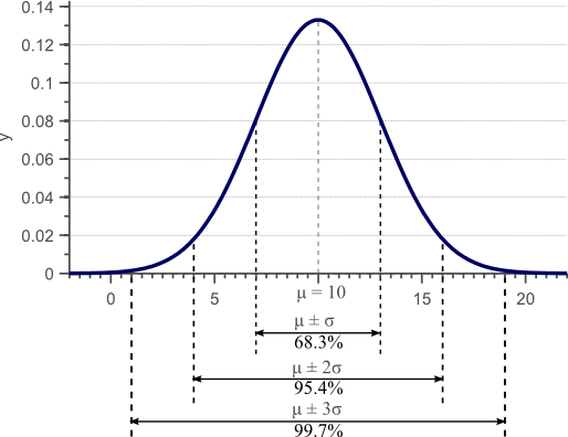
Figure 1. Gaussian density function. For normally distributed data, 68% of the samples fall within the interval defined by the mean plus and minus the standard deviation.
Usually we do not have access to the complete population of the data. In the above example, we would typically have a few observations at our disposal but we do not have access to all possible observations that define the x-axis of the plot. For example, we might have the following set of observations:
| Observation ID | Observed Value |
|---|---|
| Observation 1 | 10 |
| Observation 2 | 12 |
| Observation 3 | 7 |
| Observation 4 | 5 |
| Observation 5 | 11 |
If we now calculate the empirical mean by summing up all values and dividing by the number of observations, we have:
(1) ![]()
Usually we assume that the empirical mean is close to the actually unknown mean of the distribution, and thus assume that the observed data is sampled from a Gaussian distribution with mean ![]() . In this example, the actual mean of the distribution is 10, so the empirical mean indeed is close to the actual mean.
. In this example, the actual mean of the distribution is 10, so the empirical mean indeed is close to the actual mean.
The variance of the data is calculated as follows:
(2) 
Again, we usually assume that this empirical variance is close to the real and unknown variance of underlying distribution. In this example, the real variance was 9, so indeed the empirical variance is close to the real variance.
The question at hand is now why the formulas used to calculate the empirical mean and the empirical variance are correct. In fact, another often used formula to calculate the variance, is defined as follows:
(3) 
The only difference between equation (2) and (3) is that the former divides by N-1, whereas the latter divides by N. Both formulas are actually correct, but when to use which one depends on the situation.
In the following sections, we will completely derive the formulas that best approximate the unknown variance and mean of a normal distribution, given a few samples from this distribution. We will show in which cases to divide the variance by N and in which cases to normalize by N-1.
A formula that approximates a parameter (mean or variance) is called an estimator. In the following, we will denote the real and unknown parameters of the distribution by ![]() and
and ![]() . The estimators, e.g. the empirical average and empirical variance, are denoted as
. The estimators, e.g. the empirical average and empirical variance, are denoted as ![]() and
and ![]() .
.
To find the optimal estimators, we first need an analytical expression for the likelihood of observing a specific data point ![]() , given the fact that the population is normally distributed with a given mean
, given the fact that the population is normally distributed with a given mean ![]() and standard deviation
and standard deviation ![]() . A normal distribution with known parameters is usually denoted as
. A normal distribution with known parameters is usually denoted as ![]() . The likelihood function is then:
. The likelihood function is then:
(4) 
To calculate the mean and variance, we obviously need more than one sample from this distribution. In the following, let vector ![]() be a vector that contains all the available samples (e.g. all the values from the example in table 1). If all these samples are statistically independent, we can write their joint likelihood function as the sum of all individual likelihoods:
be a vector that contains all the available samples (e.g. all the values from the example in table 1). If all these samples are statistically independent, we can write their joint likelihood function as the sum of all individual likelihoods:
(5) 
Plugging equation (4) into equation (5) then yields an analytical expression for this joint probability density function:
(6) 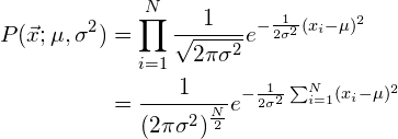
Equation (6) will be important in the next sections and will be used to derive the well known expressions for the estimators of the mean and the variance of a Gaussian distribution.
Minimum variance, unbiased estimators
To determine if an estimator is a ‘good’ estimator, we first need to define what a ‘good’ estimator really is. The goodness of an estimator depends on two measures, namely its bias and its variance (yes, we will talk about the variance of the mean-estimator and the variance of the variance-estimator). Both measures are briefly discussed in this section.
Parameter bias
Imagine that we could obtain different (disjoint) subsets of the complete population. In analogy to our previous example, imagine that, apart from the data in Table 1, we also have a Table 2 and a Table 3 with different observations. Then a good estimator for the mean, would be an estimator that on average would be equal to the real mean. Although we can live with the idea that the empirical mean from one subset of data is not equal to the real mean like in our example, a good estimator should make sure that the average of the estimated means from all subsets is equal to the real mean. This constraint is expressed mathematically by stating that the Expected Value of the estimator should equal the real parameter value:
(7) ![Rendered by QuickLaTeX.com \begin{align*} &E[\mu] = \hat{\mu}\\ &E[\sigma^2] = \hat{\sigma^2} \end{align*}](https://www.visiondummy.com/wp-content/ql-cache/quicklatex.com-b680d42fd3ce7fee8c4f6517ddd92817_l3.png)
If the above conditions hold, then the estimators are called ‘unbiased estimators’. If the conditions do not hold, the estimators are said to be ‘biased’, since on average they will either underestimate or overestimate the true value of the parameter.
Parameter variance
Unbiased estimators guarantee that on average they yield an estimate that equals the real parameter. However, this does not mean that each estimate is a good estimate. For instance, if the real mean is 10, an unbiased estimator could estimate the mean as 50 on one population subset and as -30 on another subset. The expected value of the estimate would then indeed be 10, which equals the real parameter, but the quality of the estimator clearly also depends on the spread of each estimate. An estimator that yields the estimates (10, 15, 5, 12, 8) for five different subsets of the population is unbiased just like an estimator that yields the estimates (50, -30, 100, -90, 10). However, all estimates from the first estimator are closer to the true value than those from the second estimator.
Therefore, a good estimator not only has a low bias, but also yields a low variance. This variance is expressed as the mean squared error of the estimator:
![Rendered by QuickLaTeX.com \begin{align*} &Var(\mu) = E[(\hat{\mu} - \mu)^2]\\ &Var(\sigma^2) = E[(\hat{\sigma} - \sigma)^2] \end{align*}](https://www.visiondummy.com/wp-content/ql-cache/quicklatex.com-6b784d7989b829ef1bc2a7fc555316b1_l3.png)
A good estimator is therefore is a low bias, low variance estimator. The optimal estimator, if such estimator exists, is then the one that has no bias and a variance that is lower than any other possible estimator. Such an estimator is called the minimum variance, unbiased (MVU) estimator. In the next section, we will derive the analytical expressions for the mean and the variance estimators of a Gaussian distribution. We will show that the MVU estimator for the variance of a normal distribution requires us to divide the variance by ![]() under certain assumptions, and requires us to divide by N-1 if these assumptions do not hold.
under certain assumptions, and requires us to divide by N-1 if these assumptions do not hold.
Maximum Likelihood estimation
Although numerous techniques can be used to obtain an estimator of the parameters based on a subset of the population data, the simplest of all is probably the maximum likelihood approach.
The probability of observing ![]() was defined by equation (6) as
was defined by equation (6) as ![]() . If we fix
. If we fix ![]() and
and ![]() in this function, while letting
in this function, while letting ![]() vary, we obtain the Gaussian distribution as plotted by figure 1. However, we could also choose a fixed
vary, we obtain the Gaussian distribution as plotted by figure 1. However, we could also choose a fixed ![]() and let
and let ![]() and/or
and/or ![]() vary. For example, we can choose
vary. For example, we can choose ![]() like in our previous example. We also choose a fixed
like in our previous example. We also choose a fixed ![]() , and we let
, and we let ![]() vary. Figure 2 shows the plot of each different value of
vary. Figure 2 shows the plot of each different value of ![]() for the distribution with the proposed fixed
for the distribution with the proposed fixed ![]() and
and ![]() :
:
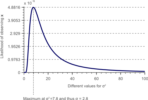
Figure 2. This plot shows the likelihood of observing fixed data ![]() if the data is normally distributed with a chosen, fixed
if the data is normally distributed with a chosen, fixed ![]() , plotted against various values of a varying
, plotted against various values of a varying ![]() .
.
In the above figure, we calculated the likelihood ![]() by varying
by varying ![]() for a fixed
for a fixed ![]() . Each point in the resulting curve represents the likelihood that observation
. Each point in the resulting curve represents the likelihood that observation ![]() is a sample from a Gaussian distribution with parameter
is a sample from a Gaussian distribution with parameter ![]() . The parameter value that corresponds to the highest likelihood is then most likely the parameter that defines the distribution our data originated from. Therefore, we can determine the optimal
. The parameter value that corresponds to the highest likelihood is then most likely the parameter that defines the distribution our data originated from. Therefore, we can determine the optimal ![]() by finding the maximum in this likelihood curve. In this example, the maximum is at
by finding the maximum in this likelihood curve. In this example, the maximum is at ![]() , such that the standard deviation is
, such that the standard deviation is ![]() . Indeed if we would calculate the variance in the traditional way, with a given
. Indeed if we would calculate the variance in the traditional way, with a given ![]() , we would find that it is equal to 7.8:
, we would find that it is equal to 7.8:

Therefore, the formula to compute the variance based on the sample data is simply derived by finding the peak of the maximum likelihood function. Furthermore, instead of fixing ![]() , we let both
, we let both ![]() and
and ![]() vary at the same time. Finding both estimators then corresponds to finding the maximum in a two-dimensional likelihood function.
vary at the same time. Finding both estimators then corresponds to finding the maximum in a two-dimensional likelihood function.
To find the maximum of a function, we simply set its derivative to zero. If we want to find the maximum of a function with two variables, we calculate the partial derivative towards each of these variables and set both to zero. In the following, let ![]() be the optimal estimator for the population mean as obtained using the maximum likelihood method, and let
be the optimal estimator for the population mean as obtained using the maximum likelihood method, and let ![]() be the optimal estimator for the variance. To maximize the likelihood function we simply calculate its (partial) derivatives and set them to zero as follows:
be the optimal estimator for the variance. To maximize the likelihood function we simply calculate its (partial) derivatives and set them to zero as follows:

and

In the following paragraphs we will use this technique to obtain the MVU estimators of both ![]() and
and ![]() . We consider two cases:
. We consider two cases:
The first case assumes that the true mean of the distribution ![]() is known. Therefore, we only need to estimate the variance and the problem then corresponds to finding the maximum in a one-dimensional likelihood function, parameterized by
is known. Therefore, we only need to estimate the variance and the problem then corresponds to finding the maximum in a one-dimensional likelihood function, parameterized by ![]() . Although this situation does not occur often in practice, it definitely has practical applications. For instance, if we know that a signal (e.g. the color value of a pixel in an image) should have a specific value, but the signal has been polluted by white noise (Gaussian noise with zero mean), then the mean of the distribution is known and we only need to estimate the variance.
. Although this situation does not occur often in practice, it definitely has practical applications. For instance, if we know that a signal (e.g. the color value of a pixel in an image) should have a specific value, but the signal has been polluted by white noise (Gaussian noise with zero mean), then the mean of the distribution is known and we only need to estimate the variance.
The second case deals with the situation where both the true mean and the true variance are unknown. This is the case you would encounter most and where you would obtain an estimate of the mean and the variance based on your sample data.
In the next paragraphs we will show that each case results in a different MVU estimator. More specific, the first case requires the variance estimator to be normalized by ![]() to be MVU, whereas the second case requires division by
to be MVU, whereas the second case requires division by ![]() to be MVU.
to be MVU.
Estimating the variance if the mean is known
Parameter estimation
If the true mean of the distribution is known, then the likelihood function is only parameterized on ![]() . Obtaining the maximum likelihood estimator then corresponds to solving:
. Obtaining the maximum likelihood estimator then corresponds to solving:
(8) ![]()
However, calculating the derivative of ![]() , defined by equation (6) is rather involved due to the exponent in the function. In fact, it is much easier to maximize the log-likelihood function instead of the likelihood function itself. Since the logarithm is a monotonous function, the maximum will be the same. Therefore, we solve the following problem instead:
, defined by equation (6) is rather involved due to the exponent in the function. In fact, it is much easier to maximize the log-likelihood function instead of the likelihood function itself. Since the logarithm is a monotonous function, the maximum will be the same. Therefore, we solve the following problem instead:
(9) ![]()
In the following we set ![]() to obtain a simpler notation. To find the maximum of the log-likelihood function, we simply calculate the derivative of the logarithm of equation (6) and set it to zero:
to obtain a simpler notation. To find the maximum of the log-likelihood function, we simply calculate the derivative of the logarithm of equation (6) and set it to zero:
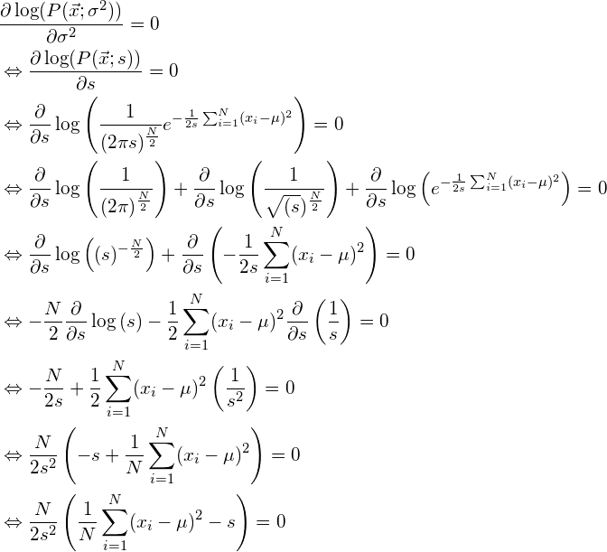
It is clear that if ![]() , then the only possible solution to the above is:
, then the only possible solution to the above is:
(10) 
Note that this maximum likelihood estimator for ![]() is indeed the traditional formula to calculate the variance of normal data. The normalization factor is
is indeed the traditional formula to calculate the variance of normal data. The normalization factor is ![]() .
.
However, the maximum likelihood method does not guarantee to deliver an unbiased estimator. On the other hand, if the obtained estimator is unbiased, then the maximum likelihood method does guarantee that the estimator is also minimum variance and thus MVU. Therefore, we need to check if the estimator in equation (10) is unbiassed.
Performance evaluation
To check if the estimator defined by equation (10) is unbiassed, we need to check if the condition of equation (7) holds, and thus if
![]()
To do this, we plug equation (10) into ![]() and write:
and write:
![Rendered by QuickLaTeX.com \begin{align*} E[s] &= E \left[\frac{1}{N}\sum_{i=1}^N(x_i - \mu)^2 \right] = \frac{1}{N} \sum_{i=1}^N E \left[(x_i - \mu)^2 \right] = \frac{1}{N} \sum_{i=1}^N E \left[x_i^2 - 2x_i \mu + \mu^2 \right]\\ &= \frac{1}{N} \left( N E[x_i^2] -2N \mu E[x_i] + N \mu^2 \right) \\ &= \frac{1}{N} \left( N E[x_i^2] -2N \mu^2 + N \mu^2 \right) \\ &= \frac{1}{N} \left( N E[x_i^2] -N \mu^2 \right) \\ \end{align*}](https://www.visiondummy.com/wp-content/ql-cache/quicklatex.com-8d2b98eefa222881e6ec5bef1a6e3c1d_l3.png)
Furthermore, an important property of variance is that the true variance ![]() can be written as
can be written as ![]() such that
such that ![]() . Using this property in the above equation yields:
. Using this property in the above equation yields:
![Rendered by QuickLaTeX.com \begin{align*} E[s] &= \frac{1}{N} \left( N E[x_i^2] -N \mu^2 \right) \\ &= \frac{1}{N} \left( N \hat{s} + N \mu^2 -N \mu^2 \right)\\ &= \frac{1}{N} \left( N \hat{s} \right)\\ &= \hat{s} \end{align*}](https://www.visiondummy.com/wp-content/ql-cache/quicklatex.com-e2fb81365c1bace2e3d216b7ee597c72_l3.png)
Since ![]() , the condition shown by equation (7) holds, and therefore the obtained estimator for the variance
, the condition shown by equation (7) holds, and therefore the obtained estimator for the variance ![]() of the data is unbiassed. Furthermore, because the maximum likelihood method guarantees that an unbiased estimator is also minimum variance (MVU), this means that no other estimator exists that can do better than the one obtained here.
of the data is unbiassed. Furthermore, because the maximum likelihood method guarantees that an unbiased estimator is also minimum variance (MVU), this means that no other estimator exists that can do better than the one obtained here.
Therefore, we have to divide by ![]() instead of
instead of ![]() while calculating the variance of normally distributed data, if the true mean of the underlying distribution is known.
while calculating the variance of normally distributed data, if the true mean of the underlying distribution is known.
Estimating the variance if the mean is unknown
Parameter estimation
In the previous section, the true mean of the distribution was known, such that we only had to find an estimator for the variance of the data. However, if the true mean is not known, then an estimator has to be found for the mean too. Furthermore, this mean estimate is used by the variance estimator. As a result, we will show that the earlier obtained estimator for the variance is no longer unbiassed. Furthermore, we will show that we can ‘unbias’ the estimator in this case by dividing by ![]() instead of by
instead of by ![]() , which slightly increases the variance of the estimator.
, which slightly increases the variance of the estimator.
As before, we use the maximum likelihood method to obtain the estimators based on the log-likelihood function. We first find the ML estimator for ![]() :
:
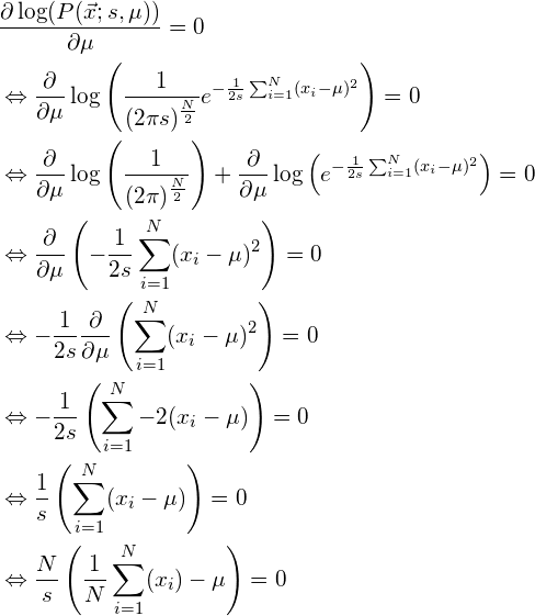
If ![]() , then it is clear that the above equation only has a solution if:
, then it is clear that the above equation only has a solution if:
(11) 
Note that indeed this is the well known formula to calculate the mean of a distribution. Although we all knew this formula, we now proved that it is the maximum likelihood estimator for the true and unknown mean ![]() of a normal distribution. For now, we will just assume that the estimator that we found earlier for the variance
of a normal distribution. For now, we will just assume that the estimator that we found earlier for the variance ![]() , defined by equation (10), is still the MVU variance estimator. In the next section however, we will show that this estimator is no longer unbiased now.
, defined by equation (10), is still the MVU variance estimator. In the next section however, we will show that this estimator is no longer unbiased now.
Performance evaluation
To check if the estimator ![]() for the true mean
for the true mean ![]() is unbiassed, we have to make sure that the condition of equation (7) holds:
is unbiassed, we have to make sure that the condition of equation (7) holds:
![Rendered by QuickLaTeX.com \begin{equation*} E[\mu] = E \left[\frac{1}{N} \sum_{i=1}^N (x_i) \right] = \frac{1}{N}\sum_{i=1}^N E[x_i] = \frac{1}{N} N E[x_i] = \frac{1}{N} N \hat{\mu} = \hat{\mu}. \end{equation*}](https://www.visiondummy.com/wp-content/ql-cache/quicklatex.com-76f691aa17482e81c9d29ac5161d991c_l3.png)
Since ![]() , this means that the obtained estimator for the mean of the distribution is unbiassed. Since the maximum likelihood method guarantees to deliver the minimum variance estimator if the estimator is unbiassed, we proved that
, this means that the obtained estimator for the mean of the distribution is unbiassed. Since the maximum likelihood method guarantees to deliver the minimum variance estimator if the estimator is unbiassed, we proved that ![]() is the MVU estimator of the mean.
is the MVU estimator of the mean.
To check if the earlier found estimator ![]() for the variance
for the variance ![]() is still unbiassed if it is based on the empirical mean
is still unbiassed if it is based on the empirical mean ![]() instead of the true mean
instead of the true mean ![]() , we simply plug the obtained estimator
, we simply plug the obtained estimator ![]() into the earlier derived estimator
into the earlier derived estimator ![]() of equation (10):
of equation (10):
![Rendered by QuickLaTeX.com \begin{align*} s &= \sigma^2 = \frac{1}{N}\sum_{i=1}^N(x_i - \mu)^2\\ &=\frac{1}{N}\sum_{i=1}^N \left(x_i - \frac{1}{N} \sum_{i=1}^N (x_i) \right)^2\\ &=\frac{1}{N}\sum_{i=1}^N \left[x_i^2 - 2 x_i \frac{1}{N} \sum_{i=1}^N (x_i) + \left(\frac{1}{N} \sum_{i=1}^N (x_i) \right)^2 \right]\\ &=\frac{\sum_{i=1}^N x_i^2}{N} - \frac{2\sum_{i=1}^N x_i \sum_{i=1}^N x_i}{N^2} + \left(\frac{\sum_{i=1}^N x_i}{N} \right)^2\\ &=\frac{\sum_{i=1}^N x_i^2}{N} - \frac{2\sum_{i=1}^N x_i \sum_{i=1}^N x_i}{N^2} + \left(\frac{\sum_{i=1}^N x_i}{N} \right)^2\\ &=\frac{\sum_{i=1}^N x_i^2}{N} - \left(\frac{\sum_{i=1}^N x_i}{N} \right)^2\\ \end{align*}](https://www.visiondummy.com/wp-content/ql-cache/quicklatex.com-8804df142d23349705e2b2bae64d5378_l3.png)
To check if the estimator is still unbiased, we now need to check again if the condition of equation (7) holds:
![Rendered by QuickLaTeX.com \begin{align*} E[s] &= E \left[ \frac{\sum_{i=1}^N x_i^2}{N} - \left(\frac{\sum_{i=1}^N x_i}{N} \right)^2 \right ] \\ & = \frac{\sum_{i=1}^N E[x_i^2]}{N} - \frac{E[(\sum_{i=1}^N x_i)^2]}{N^2} \\ \end{align*}](https://www.visiondummy.com/wp-content/ql-cache/quicklatex.com-7acd92c866aa7af2c56a2477e32f0797_l3.png)
As mentioned in the previous section, an important property of variance is that the true variance ![]() can be written as
can be written as ![]() such that
such that ![]() . Using this property in the above equation yields:
. Using this property in the above equation yields:
![Rendered by QuickLaTeX.com \begin{align*} E[s] &= \frac{\sum_{i=1}^N E[x_i^2]}{N} - \frac{E[(\sum_{i=1}^N x_i)^2]}{N^2} \\ &= s + \mu^2 - \frac{E[(\sum_{i=1}^N x_i)^2]}{N^2} \\ &= s + \mu^2 - \frac{E[\sum_{i=1}^N x_i^2 + \sum_i^N \sum_{j\neq i}^N x_i x_j]}{N^2} \\ &= s + \mu^2 - \frac{E[N(s+\mu^2) + \sum_i^N \sum_{j\neq i}^N x_i x_j]}{N^2} \\ &= s + \mu^2 - \frac{N(s+\mu^2) + \sum_i^N \sum_{j\neq i}^N E[x_i] E[x_j]}{N^2} \\ &= s + \mu^2 - \frac{N(s+\mu^2) + N(N-1)\mu^2}{N^2} \\ &= s + \mu^2 - \frac{N(s+\mu^2) + N^2\mu^2 -N\mu^2}{N^2} \\ &= s + \mu^2 - \frac{s+\mu^2 + N\mu^2 -\mu^2}{N} \\ &= s + \mu^2 - \frac{s}{N} - \frac{\mu^2}{N} - \mu^2 + \frac{\mu^2}{N}\\ &= s - \frac{s}{N}\\ &= s \left( 1 - \frac{1}{N} \right)\\ &= s \left(\frac{N-1}{N} \right) \end{align*}](https://www.visiondummy.com/wp-content/ql-cache/quicklatex.com-322edfb0546fa23a9df81283b7593cfe_l3.png)
Since clearly ![]() , this shows that estimator for the variance of the distribution is no longer unbiassed. In fact, this estimator on average underestimates the true variance with a factor
, this shows that estimator for the variance of the distribution is no longer unbiassed. In fact, this estimator on average underestimates the true variance with a factor ![]() . As the number of samples approaches infinity (
. As the number of samples approaches infinity (![]() ), this bias converges to zero. For small sample sets however, the bias is signification and should be eliminated.
), this bias converges to zero. For small sample sets however, the bias is signification and should be eliminated.
Fixing the bias
Since the bias is merely a factor, we can eliminate it by scaling the biased estimator ![]() defined by equation (10) by the inverse of the bias. We therefore define a new, unbiased estimate
defined by equation (10) by the inverse of the bias. We therefore define a new, unbiased estimate ![]() as follows:
as follows:
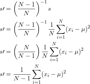
This estimator is now unbiassed and indeed resembles the traditional formula to calculate the variance, where we divide by ![]() instead of
instead of ![]() . However, note that the resulting estimator is no longer the minimum variance estimator, but it is the estimator with the minimum variance amongst all unbiased estimators. If we divide by
. However, note that the resulting estimator is no longer the minimum variance estimator, but it is the estimator with the minimum variance amongst all unbiased estimators. If we divide by ![]() , then the estimator is biassed, and if we divide by
, then the estimator is biassed, and if we divide by ![]() , the estimator is not the minimum variance estimator. However, in general having a biased estimator is much worse than having a slightly higher variance estimator. Therefore, if the mean of the population is unknown, division by
, the estimator is not the minimum variance estimator. However, in general having a biased estimator is much worse than having a slightly higher variance estimator. Therefore, if the mean of the population is unknown, division by ![]() should be used instead of division by
should be used instead of division by ![]() .
.
Conclusion
In this article, we showed where the usual formulas for calculating the mean and the variance of normally distributed data come from. Furthermore, we have proven that the normalization factor in the variance estimator formula should be ![]() if the true mean of the population is known, and should be
if the true mean of the population is known, and should be ![]() if the mean itself also has to be estimated.
if the mean itself also has to be estimated.
If you’re new to this blog, don’t forget to subscribe, or follow me on twitter!


This is the first proof for the unbiased estimators of variance and mean that I actually understand! Thank you so much for your great blog
I am pretty sure that the description for [6] is not correct – the pdf of the Gaussian does not actually give you the probability of x
Hi Brian, tnx for your feedback. However, I’m not sure what you mean. The PDF actually does represent the probability of observing x. Obviously, since x is continuous, you need to integrate the PDF over a small interval surrounding x to obtain the actual probability.
That was my only point, that calling [4] a probability (as in “The probability of observing a point x….”) is not technically correct – for that reason you mentioned.
Thanks again, Brian. Talking about likelihood functions instead of probabilities is probably more accurate in this context indeed, so I changed it.
I was looking for this proof for so long. Thanks for sharing.
Hi Vincent
Thanks for the awesome work. I’ve enjoyed a number of your articles so far!
I am writing to let you know about an awesome book called “Probability Theory: The Logic of Science” by ET Jaynes. Chapter 17 in that book has a great section on the pathologies of unbiased estimators in general. He goes on to show that the optimal estimator (in the minimum mean square error sense) is the first moment of the posterior distribution (which you may want to marginalise if you are only interested in one of the parameters).
Long story short, there is a serious problem with using your unbiased estimator for the variance, especially for non-gaussian sampling distributions. The variance of the estimator is worsened by using the N/(N-1) multiplicative correction to equation (3) in your article. That is to say that you can do better (in the mean square error sense) than equation (2) if you are considering the class of multiplicative corrections to estimate the variance from equation (3).
Let me know if you’d like more details.
Hi Jacques, thanks for your comment. I will defintely have a look at the book you mentioned! Although it is true that the variance of the estimator increases a bit by introducing Bessel’s correction, a slight increase in variance is often prefered over a biassed estimator. However, as you mention, it is indeed important to consider the Gaussian assumptions in the above derivations. For non-Gaussian distributions you might indeed want to considere different options, but then again the variance is usually not a very interesting statistic for non-Gaussian distributions. Thanks again for your valuable feedback!
Thanks a lot for the wonderful post.
Just one clarification : shouldn’t it be underestimates the true variance by a factor of n-1/n rather than overestimates ?
Obviously you are right, Tushant. Thanks for your input! I just fixed this typo.
Thanks very much. Beautiful post. It’s not easy to find why you have to divide the sample variance by n-1, on many statistics books….!
Bye.
Hi Vincent, this is a really great article… Well written and nicely explained!
Just a small typo I found: In the section “Estimating the variance if the mean is unknown”, subsection “Parameter estimation” in the third equation there is missing an s in the denominator of the first log-summand. Not a big thing, since it is eliminated anyways but just wanted to let you know.
Hi Vincent,
can you please give a proof that the maximum likelihood method guarantees an unbiased estimator is also minimum variance?
Nicely written article, but I think you are super confused about your “hat” notation. In Statistics, the hat is reserved to denote the estimator or the estimate (depending on the context), whereas without a hat is the population parameter. In your equation (4) mu and sigma are clearly the parameters of the normal distribution, however in the preceding paragraph you say these are estimators, namely the empirical average and empirical variance.
Check “we can write their joint likelihood function as the sum of all individual likelihoods…” directly before equation 5. I think it should read “the product of individual likelihoods” instead of sum.
Thank you for your articles, I have found them very helpful.
Outstanding explanation of one of the “mysteries” of statistics that has long defied a good explanation. Thanks for taking the time to post.
Hi, there, I like your essay very much. I hope you do not mind that I have translated your article to Chinese.
Here is the link: http://commanber.com/2017/06/17/sample-variance/
I will remove my article immediately if you do not allow me to release the Chinese version of your article.
Thanks very much!
Have a good day!
Hi Michael, it’s an honor, great work! Thanks a lot!