What are eigenvectors and eigenvalues?
Contents
Introduction
Eigenvectors and eigenvalues have many important applications in computer vision and machine learning in general. Well known examples are PCA (Principal Component Analysis) for dimensionality reduction or EigenFaces for face recognition. An interesting use of eigenvectors and eigenvalues is also illustrated in my post about error ellipses. Furthermore, eigendecomposition forms the base of the geometric interpretation of covariance matrices, discussed in an more recent post. In this article, I will provide a gentle introduction into this mathematical concept, and will show how to manually obtain the eigendecomposition of a 2D square matrix.
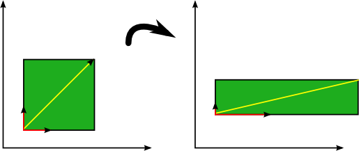
An eigenvector is a vector whose direction remains unchanged when a linear transformation is applied to it. Consider the image below in which three vectors are shown. The green square is only drawn to illustrate the linear transformation that is applied to each of these three vectors.

Eigenvectors (red) do not change direction when a linear transformation (e.g. scaling) is applied to them. Other vectors (yellow) do.
The transformation in this case is a simple scaling with factor 2 in the horizontal direction and factor 0.5 in the vertical direction, such that the transformation matrix ![]() is defined as:
is defined as:
 .
.
A vector ![]() is then scaled by applying this transformation as
is then scaled by applying this transformation as ![]() . The above figure shows that the direction of some vectors (shown in red) is not affected by this linear transformation. These vectors are called eigenvectors of the transformation, and uniquely define the square matrix
. The above figure shows that the direction of some vectors (shown in red) is not affected by this linear transformation. These vectors are called eigenvectors of the transformation, and uniquely define the square matrix ![]() . This unique, deterministic relation is exactly the reason that those vectors are called ‘eigenvectors’ (Eigen means ‘specific’ in German).
. This unique, deterministic relation is exactly the reason that those vectors are called ‘eigenvectors’ (Eigen means ‘specific’ in German).
In general, the eigenvector ![]() of a matrix
of a matrix ![]() is the vector for which the following holds:
is the vector for which the following holds:
(1) ![]()
where ![]() is a scalar value called the ‘eigenvalue’. This means that the linear transformation
is a scalar value called the ‘eigenvalue’. This means that the linear transformation ![]() on vector
on vector ![]() is completely defined by
is completely defined by ![]() .
.
We can rewrite equation (1) as follows:
(2) 
where ![]() is the identity matrix of the same dimensions as
is the identity matrix of the same dimensions as ![]() .
.
However, assuming that ![]() is not the null-vector, equation (2) can only be defined if
is not the null-vector, equation (2) can only be defined if ![]() is not invertible. If a square matrix is not invertible, that means that its determinant must equal zero. Therefore, to find the eigenvectors of
is not invertible. If a square matrix is not invertible, that means that its determinant must equal zero. Therefore, to find the eigenvectors of ![]() , we simply have to solve the following equation:
, we simply have to solve the following equation:
(3) ![]()
In the following sections we will determine the eigenvectors and eigenvalues of a matrix ![]() , by solving equation (3). Matrix
, by solving equation (3). Matrix ![]() in this example, is defined by:
in this example, is defined by:
(4) 
Calculating the eigenvalues
To determine the eigenvalues for this example, we substitute ![]() in equation (3) by equation (4) and obtain:
in equation (3) by equation (4) and obtain:
(5) 
Calculating the determinant gives:
(6) 
To solve this quadratic equation in ![]() , we find the discriminant:
, we find the discriminant:
![]()
Since the discriminant is strictly positive, this means that two different values for ![]() exist:
exist:
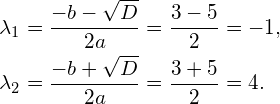
(7) 
We have now determined the two eigenvalues ![]() and
and ![]() . Note that a square matrix of size
. Note that a square matrix of size ![]() always has exactly
always has exactly ![]() eigenvalues, each with a corresponding eigenvector. The eigenvalue specifies the size of the eigenvector.
eigenvalues, each with a corresponding eigenvector. The eigenvalue specifies the size of the eigenvector.
Calculating the first eigenvector
We can now determine the eigenvectors by plugging the eigenvalues from equation (7) into equation (1) that originally defined the problem. The eigenvectors are then found by solving this system of equations.
We first do this for eigenvalue ![]() , in order to find the corresponding first eigenvector:
, in order to find the corresponding first eigenvector:

Since this is simply the matrix notation for a system of equations, we can write it in its equivalent form:
(8) 
and solve the first equation as a function of ![]() , resulting in:
, resulting in:
(9) ![]()
Since an eigenvector simply represents an orientation (the corresponding eigenvalue represents the magnitude), all scalar multiples of the eigenvector are vectors that are parallel to this eigenvector, and are therefore equivalent (If we would normalize the vectors, they would all be equal). Thus, instead of further solving the above system of equations, we can freely chose a real value for either ![]() or
or ![]() , and determine the other one by using equation (9).
, and determine the other one by using equation (9).
For this example, we arbitrarily choose ![]() , such that
, such that ![]() . Therefore, the eigenvector that corresponds to eigenvalue
. Therefore, the eigenvector that corresponds to eigenvalue ![]() is
is
(10) 
Calculating the second eigenvector
Calculations for the second eigenvector are similar to those needed for the first eigenvector;
We now substitute eigenvalue ![]() into equation (1), yielding:
into equation (1), yielding:
(11) 
Written as a system of equations, this is equivalent to:
(12) 
Solving the first equation as a function of ![]() resuls in:
resuls in:
(13) ![]()
We then arbitrarily choose ![]() , and find
, and find ![]() . Therefore, the eigenvector that corresponds to eigenvalue
. Therefore, the eigenvector that corresponds to eigenvalue ![]() is
is
(14) 
Conclusion
In this article we reviewed the theoretical concepts of eigenvectors and eigenvalues. These concepts are of great importance in many techniques used in computer vision and machine learning, such as dimensionality reduction by means of PCA, or face recognition by means of EigenFaces.
If you’re new to this blog, don’t forget to subscribe, or follow me on twitter!


You managed to explain that in plain English. Very nice article. Thank you.
Trivial thing: I think the subscripts on x11 and x12 on [13] and [14] should be x21 and x22.
Thanks for noticing, Khon! I fixed the typo.
Nice Article
I like your blog.I enjoyed reading your blog.It was amazing.Thanks a lot.
Great post! In equation 2 implication, shouldn’t the vector v post-multiply (A – \lambda I) since matrix multiplication is non-commutative? I.e., (A – \lambda I) v = 0 rather than v (A – \lambda I) = 0.
Great writing it is such a cool and nice idea thanks for sharing your post . I like your post very much. Thanks for your post.
Think you may now have x_21 and x_22 the wrong way round in eqn [13] and have subsequent corrections to be made thereafter. Very helpful piece though.
Very nice article! I have a question. You wrote “However, assuming that vec is not the null-vector, equation (2) can only be defined if (A – lambda I) is not invertible.”
Could you explain that a bit more? What will happen if (A – lambda I) is invertible?
I was also confused about this. After researching for a good hour or two on determinants and invertible matrices, I think it’s safe to say that a non-invertible matrix either:
– Has a row (or column) with all zeros
– Has at least two rows (or columns) that are equivalent.
The underlying reason for this (and its correlation with determinants) is that the determinant of a matrix is essentially the area in R^n space of the columns of the matrix (see http://math.stackexchange.com/questions/668/whats-an-intuitive-way-to-think-about-the-determinant).
So, if two of the columns of the matrix are equivalent, that means that they’re parallel, and the area of the parallelepiped formed has an area of zero. (It would also have an area of zero if one of the vectors is a null-vector).
So I think the reason is that, unless v is the null-vector of all zeros, one of the above properties is necessary for a linear combination of the rows to add up to zero (This is the part I’m unsure about, because the dimensions of equation (2) isn’t 1×1, is it?).
If someone actually knows what they’re talking about, please correct me. This is just my understanding after googling some stuff.
Hey that’s great stuff! It helped me a lot to get things clear in my mind. Please go on! BTW typo: Eq. 6: I think it should be +lambda-square not *minus* lambda-square. Thanks, Sebastian
Another Trivial Thing: I think x22 = 2/3 x21 on [13]
Thanks for your explicit explanation.
Hi Vincent,
Thank you for writing such nice articles.
I have a question for you. In the post you have written that ” Since an eigenvector simply represents an orientation”.
When you say something as a “Vector” it means that it has both direction and magnitude. But this statement was confusing for me.
Can you please explain what do you mean by this statement?
Thank you
Nrupatunga
Hi Nrupatunga,
Usually, we normalize the eigenvector such that its magnitude is one. In this case, the eigenvector only represents a direction, whereas its corresponding eigenvalue represents its magnitude.
Thank you Mr Vincent, I as well thought this is what you meant. Hope that wasn’t silly to ask.
Thank you for making it clear to me that its just mathematical manipulations.
Your blog is very neatly maintained. I would be very happy to learn more from you through your articles.
Thank you
thanks and so great
Nice article. But I guess there is error in calculating second eigen vector. It should 2 3 instead of 3 2. Please check at your end and let us know. Thanks in advance !! I must say it is a very well written article.
plz can u descibe its use in one application
Great explanation.
It looks like there is a typo in the 2nd line while deriving equation (6). The lambda square should have a positive sign.
Great work