
Feature extraction using PCA
Contents
Introduction
In this article, we discuss how Principal Component Analysis (PCA) works, and how it can be used as a dimensionality reduction technique for classification problems. At the end of this article, Matlab source code is provided for demonstration purposes.
In an earlier article, we discussed the so called Curse of Dimensionality and showed that classifiers tend to overfit the training data in high dimensional spaces. The question then rises which features should be preferred and which ones should be removed from a high dimensional feature vector.
If all features in this feature vector were statistically independent, one could simply eliminate the least discriminative features from this vector. The least discriminative features can be found by various greedy feature selection approaches. However, in practice, many features depend on each other or on an underlying unknown variable. A single feature could therefore represent a combination of multiple types of information by a single value. Removing such a feature would remove more information than needed. In the next paragraphs, we introduce PCA as a feature extraction solution to this problem, and introduce its inner workings from two different perspectives.
PCA as a decorrelation method
More often than not, features are correlated. As an example, consider the case where we want to use the red, green and blue components of each pixel in an image to classify the image (e.g. detect dogs versus cats). Image sensors that are most sensitive to red light also capture some blue and green light. Similarly, sensors that are most sensitive to blue and green light also exhibit a certain degree of sensitivity to red light. As a result, the R, G, B components of a pixel are statistically correlated. Therefore, simply eliminating the R component from the feature vector, also implicitly removes information about the G and B channels. In other words, before eliminating features, we would like to transform the complete feature space such that the underlying uncorrelated components are obtained.
Consider the following example of a 2D feature space:

Figure 1 2D Correlated data with eigenvectors shown in color.
The features  and
and  , illustrated by figure 1, are clearly correlated. In fact, their covariance matrix is:
![\begin{equation*} \Sigma = \begin{bmatrix} 16.87 & 14.94 \\[0.3em] 14.94 & 17.27 \\[0.3em] \end{bmatrix} \end{equation*}](https://www.visiondummy.com/wp-content/ql-cache/quicklatex.com-14c617ab0933f92980b8be162cbd2e52_l3.png "Rendered by QuickLaTeX.com")
In an earlier article we discussed the geometric interpretation of the covariance matrix. We saw that the covariance matrix can be decomposed as a sequence of rotation and scaling operations on white, uncorrelated data, where the rotation matrix is defined by the eigenvectors of this covariance matrix. Therefore, intuitively, it is easy to see that the data  shown in figure 1 can be decorrelated by rotating each data point such that the eigenvectors
  become the new reference axes:
(1) 

Figure 2.2D Uncorrelated data with eigenvectors shown in color.
The covariance matrix of the resulting data is now diagonal, meaning that the new axes are uncorrelated:
![\begin{equation*} \Sigma' = \begin{bmatrix} 1.06 & 0.0 \\[0.3em] 0.0 & 16.0 \\[0.3em] \end{bmatrix} \end{equation*}](https://www.visiondummy.com/wp-content/ql-cache/quicklatex.com-47a3fd2d5bf71c6b0cc423f4f2bddacd_l3.png "Rendered by QuickLaTeX.com")
In fact, the original data used in this example and shown by figure 1 was generated by linearly combining two 1D Gaussian feature vectors  and
and  as follows:

Since the features and are linear combinations of some unknown underlying components  and
and  , directly eliminating either or as a feature would have removed some information from both and . Instead, rotating the data by the eigenvectors of its covariance matrix, allowed us to directly recover the independent components and (up to a scaling factor). This can be seen as follows: The eigenvectors of the covariance matrix of the original data are (each column represents an eigenvector):
![\begin{equation*} V = \begin{bmatrix} -0.7071 & 0.7071 \\[0.3em] 0.7071 & 0.7071 \\[0.3em] \end{bmatrix} \end{equation*}](https://www.visiondummy.com/wp-content/ql-cache/quicklatex.com-5118e8d82d044ca6a8c48a62c8e8659b_l3.png "Rendered by QuickLaTeX.com")
The first thing to notice is that in this case is a rotation matrix, corresponding to a rotation of 45 degrees (cos(45)=0.7071), which indeed is evident from figure 1. Secondly, treating as a linear transformation matrix results in a new coordinate system, such that each new feature  and
and  is expressed as a linear combination of the original features and :
(2) 
and
(3) 
In other words, decorrelation of the feature space corresponds to the recovery of the unknown, uncorrelated components and  of the data (up to an unknown scaling factor if the transformation matrix was not orthogonal). Once these components have been recovered, it is easy to reduce the dimensionality of the feature space by simply eliminating either or .
In the above example we started with a two-dimensional problem. If we would like to reduce the dimensionality, the question remains whether to eliminate (and thus ) or (and thus ). Although this choice could depend on many factors such as the separability of the data in case of classification problems, PCA simply assumes that the most interesting feature is the one with the largest variance or spread. This assumption is based on an information theoretic point of view, since the dimension with the largest variance corresponds to the dimension with the largest entropy and thus encodes the most information. The smallest eigenvectors will often simply represent noise components, whereas the largest eigenvectors often correspond to the principal components that define the data.
Dimensionality reduction by means of PCA is then accomplished simply by projecting the data onto the largest eigenvectors of its covariance matrix. For the above example, the resulting 1D feature space is illustrated by figure 3:

Figure 3. PCA: 2D data projected onto its largest eigenvector.
Obivously, the above example easily generalizes to higher dimensional feature spaces. For instance, in the three-dimensional case, we can either project the data onto the plane defined by the two largest eigenvectors to obtain a 2D feature space, or we can project it onto the largest eigenvector to obtain a 1D feature space. This is illustrated by figure 4:

Figure 4. 3D data projected onto a 2D or 1D linear subspace by means of Principal Component Analysis.
In general, PCA allows us to obtain a linear M-dimensional subspace of the original N-dimensional data, where  . Furthermore, if the unknown, uncorrelated components are Gaussian distributed, then PCA actually acts as an independent component analysis since uncorrelated Gaussian variables are statistically independent. However, if the underlying components are not normally distributed, PCA merely generates decorrelated variables which are not necessarily statistically independent. In this case, non-linear dimensionality reduction algorithms might be a better choice.
PCA as an orthogonal regression method
In the above discussion, we started with the goal of obtaining independent components (or at least uncorrelated components if the data is not normally distributed) to reduce the dimensionality of the feature space. We found that these so called ‘principal components’ are obtained by the eigendecomposition of the covariance matrix of our data. The dimensionality is then reduced by projecting the data onto the largest eigenvectors.
Now let’s forget about our wish to find uncorrelated components for a while. Instead, we will now try to reduce the dimensionality by finding a linear subspace of the original feature space onto which we can project our data such that the projection error is minimized. In the 2D case, this means that we try to find a vector such that projecting the data onto this vector corresponds to a projection error that is lower than the projection error that would be obtained when projecting the data onto any other possible vector. The question is then how to find this optimal vector.
Consider the example shown by figure 5. Three different projection vectors are shown, together with the resulting 1D data. In the next paragraphs, we will discuss how to determine which projection vector minimizes the projection error. Before searching for a vector that minimizes the projection error, we have to define this error function.

Figure 5 Dimensionality reduction by projection onto a linear subspace
A well known method to fit a line to 2D data is least squares regression. Given the independent variable and the dependent variable , the least squares regressor corresponds to the line  , such that the sum of the squared residual errors
  is minimized. In other words, if is treated as the independent variable, then the obtained regressor
  is a linear function that can predict the dependent variable such that the squared error is minimal. The resulting model is illustrated by the blue line in figure 5, and the error that is minimized is illustrated in figure 6.

Figure 6. Linear regression where x is the independent variable and y is the dependent variable, corresponds to minimizing the vertical projection error.
However, in the context of feature extraction, one might wonder why we would define feature as the independent variable and feature as the dependent variable. In fact, we could easily define as the independent variable and find a linear function  that predicts the dependent variable , such that
  is minimized. This corresponds to minimization of the horizontal projection error and results in a different linear model as shown by figure 7:

Figure 7. Linear regression where y is the independent variable and x is the dependent variable, corresponds to minimizing the horizontal projection error.
Clearly, the choice of independent and dependent variables changes the resulting model, making ordinary least squares regression an asymmetric regressor. The reason for this is that least squares regression assumes the independent variable to be noise-free, whereas the dependent variable is assumed to be noisy. However, in the case of classification, all features are usually noisy observations such that neither or should be treated as independent. In fact, we would like to obtain a model  that minimizes both the horizontal and the vertical projection error simultaneously. This corresponds to finding a model such that the orthogonal projection error is minimized as shown by figure 8.

Figure 8. Linear regression where both variables are independent corresponds to minimizing the orthogonal projection error.
The resulting regression is called Total Least Squares regression or orthogonal regression, and assumes that both variables are imperfect observations. An interesting observation is now that the obtained vector, representing the projection direction that minimizes the orthogonal projection error, corresponds the the largest principal component of the data:

Figure 9. The vector which the data can be projected unto with minimal orthogonal error corresponds to the largest eigenvector of the covariance matrix of the data.
In other words, if we want to reduce the dimensionality by projecting the original data onto a vector such that the squared projection error is minimized in all directions, we can simply project the data onto the largest eigenvectors. This is exactly what we called Principal Component Analysis in the previous section, where we showed that such projection also decorrelates the feature space.
A practical PCA application: Eigenfaces
Although the above examples are limited to two or three dimensions for visualization purposes, dimensionality reduction usually becomes important when the number of features is not negligible compared to the number of training samples. As an example, suppose we would like to perform face recognition, i.e. determine the identity of the person depicted in an image, based on a training dataset of labeled face images. One approach might be to treat the brightness of each pixel of the image as a feature. If the input images are of size 32×32 pixels, this means that the feature vector contains 1024 feature values. Classifying a new face image can then be done by calculating the Euclidean distance between this 1024-dimensional vector, and the feature vectors of the people in our training dataset. The smallest distance then tells us which person we are looking at.
However, operating in a 1024-dimensional space becomes problematic if we only have a few hundred training samples. Furthermore, Euclidean distances behave strangely in high dimensional spaces as discussed in an earlier article. Therefore, we could use PCA to reduce the dimensionality of the feature space by calculating the eigenvectors of the covariance matrix of the set of 1024-dimensional feature vectors, and then projecting each feature vector onto the largest eigenvectors.
Since the eigenvector of 2D data is 2-dimensional, and an eigenvector of 3D data is 3-dimensional, the eigenvectors of 1024-dimensional data is 1024-dimensional. In other words, we could reshape each of the 1024-dimensional eigenvectors to a 32×32 image for visualization purposes. Figure 10 shows the first four eigenvectors obtained by eigendecomposition of the Cambridge face dataset:
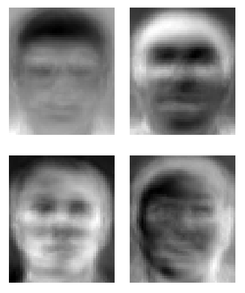
Figure 10. The four largest eigenvectors, reshaped to images, resulting in so called EigenFaces. (source: https://nl.wikipedia.org/wiki/Eigenface)
Each 1024-dimensional feature vector (and thus each face) can now be projected onto the N largest eigenvectors, and can be represented as a linear combination of these eigenfaces. The weights of these linear combinations determine the identity of the person. Since the largest eigenvectors represent the largest variance in the data, these eigenfaces describe the most informative image regions (eyes, noise, mouth, etc.). By only considering the first N (e.g. N=70) eigenvectors, the dimensionality of the feature space is greatly reduced.
The remaining question is now how many eigenfaces should be used, or in the general case; how many eigenvectors should be kept. Removing too many eigenvectors might remove important information from the feature space, whereas eliminating too few eigenvectors leaves us with the curse of dimensionality. Regrettably there is no straight answer to this problem. Although cross-validation techniques can be used to obtain an estimate of this hyperparameter, choosing the optimal number of dimensions remains a problem that is mostly solved in an empirical (an academic term that means not much more than ‘trial-and-error’) manner. Note that it is often useful to check how much (as a percentage) of the variance of the original data is kept while eliminating eigenvectors. This is done by dividing the sum of the kept eigenvalues by the sum of all eigenvalues.
The PCA recipe
Based on the previous sections, we can now list the simple recipe used to apply PCA for feature extraction:
1) Center the data
In an earlier article, we showed that the covariance matrix can be written as a sequence of linear operations (scaling and rotations). The eigendecomposition extracts these transformation matrices: the eigenvectors represent the rotation matrix, while the eigenvalues represent the scaling factors. However, the covariance matrix does not contain any information related to the translation of the data. Indeed, to represent translation, an affine transformation would be needed instead of a linear transformation.
Therefore, before applying PCA to rotate the data in order to obtain uncorrelated axes, any existing shift needs to be countered by subtracting the mean of the data from each data point. This simply corresponds to centering the data such that its average becomes zero.
2) Normalize the data
The eigenvectors of the covariance matrix point in the direction of the largest variance of the data. However, variance is an absolute number, not a relative one. This means that the variance of data, measured in centimeters (or inches) will be much larger than the variance of the same data when measured in meters (or feet). Consider the example where one feature represents the length of an object in meters, while the second feature represents the width of the object in centimeters. The largest variance, and thus the largest eigenvector, will implicitly be defined by the first feature if the data is not normalized.
To avoid this scale-dependent nature of PCA, it is useful to normalize the data by dividing each feature by its standard deviation. This is especially important if different features correspond to different metrics.
3) Calculate the eigendecomposition
Since the data will be projected onto the largest eigenvectors to reduce the dimensionality, the eigendecomposition needs to be obtained. One of the most widely used methods to efficiently calculate the eigendecomposition is Singular Value Decomposition (SVD).
4) Project the data
To reduce the dimensionality, the data is simply projected onto the largest eigenvectors. Let be the matrix whose columns contain the largest eigenvectors and let be the original data whose columns contain the different observations. Then the projected data  is obtained as
  . We can either choose the number of remaining dimensions, i.e. the columns of , directly, or we can define the amount of variance of the original data that needs to kept while eliminating eigenvectors. If only
  eigenvectors are kept, and
  represent the corresponding eigenvalues, then the amount of variance that remains after projecting the original
  -dimensional data can be calculated as:
(4) 
PCA pitfalls
In the above discussion, several assumptions have been made. In the first section, we discussed how PCA decorrelates the data. In fact, we started the discussion by expressing our desire to recover the unknown, underlying independent components of the observed features. We then assumed that our data was normally distributed, such that statistical independence simply corresponds to the lack of a linear correlation. Indeed, PCA allows us to decorrelate the data, thereby recovering the independent components in case of Gaussianity. However, it is important to note that decorrelation only corresponds to statistical independency in the Gaussian case. Consider the data obtained by sampling half a period of  :
:
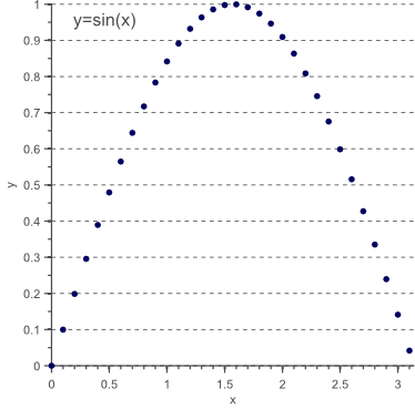
Figure 11 Uncorrelated data is only statistically independent if normally distributed. In this example a clear non-linear dependency still exists: y=sin(x).
Although the above data is clearly uncorrelated (on average, the y-value increases as much as it decreases when the x-value goes up) and therefore corresponds to a diagonal covariance matrix, there still is a clear non-linear dependency between both variables.
In general, PCA only uncorrelates the data but does not remove statistical dependencies. If the underlying components are known to be non-Gaussian, techniques such as ICA could be more interesting. On the other hand, if non-linearities clearly exist, dimensionality reduction techniques such as non-linear PCA can be used. However, keep in mind that these methods are prone to overfitting themselves, since more parameters are to be estimated based on the same amount of training data.
A second assumption that was made in this article, is that the most discriminative information is captured by the largest variance in the feature space. Since the direction of the largest variance encodes the most information this is likely to be true. However, there are cases where the discriminative information actually resides in the directions of the smallest variance, such that PCA could greatly hurt classification performance. As an example, consider the two cases of figure 12, where we reduce the 2D feature space to a 1D representation:

Figure 12. In the first case, PCA would hurt classification performance because the data becomes linearly unseparable. This happens when the most discriminative information resides in the smaller eigenvectors.
If the most discriminative information is contained in the smaller eigenvectors, applying PCA might actually worsen the Curse of Dimensionality because now a more complicated classification model (e.g. non-linear classifier) is needed to classify the lower dimensional problem. In this case, other dimensionality reduction methods might be of interest, such as Linear Discriminant Analysis (LDA) which tries to find the projection vector that optimally separates the two classes.
Source Code
The following code snippet shows how to perform principal component analysis for dimensionality reduction in Matlab:
Matlab source code
Conclusion
In this article, we discussed the advantages of PCA for feature extraction and dimensionality reduction from two different points of view. The first point of view explained how PCA allows us to decorrelate the feature space, whereas the second point of view showed that PCA actually corresponds to orthogonal regression.
Furthermore, we briefly introduced Eigenfaces as a well known example of PCA based feature extraction, and we covered some of the most important disadvantages of Principal Component Analysis.
If you’re new to this blog, don’t forget to subscribe, or follow me on twitter!


Again, Vincent — you are awesome.
You have a true talent for explaining and deconstructing things.
By the way, can you tell me what you are using for hosting your blog (platform, theme, etc)?
It’s really nicely done.
Tnx again for your nice feedback, Bryan! I’m simply using WordPress with the Magazine theme: http://www.wrock.org/product/magazine-style-theme/. I’m hosting at gigaserving.com.
Great post again, thanks
Just some typos (Below “PCA as a decorrelation method”):
More often then not, features are correlated. As an example, consider the case were we …
PCA as an orthogonal regression method makes me think of SVM.
Thanks for your feedback again! I fixed the typos.
Please share more tutorials. Your work is simply awesome.
Nicely done. Easily readable and understood by freshies like me!
Can you tell me how can i perform matching algorithm using pca?
how to extract the features in a color image using pca?
Wouah, I just discovered your blog and the articles are greats ! Like difficult concept can be easily understood. Thanks you very much Vincent.
awesome explanation… you rock…
VERY CLEAR. Very enjoyable.
Actually I have been studying in Basic Linear Algebra for 3 years, it is really rare to find summary covering names with proofs in an easy way and showing the minimum possible pictures at the right parts.
I spent some hours taking notes and even reading from wiki when you added it as note so simply I passed through all the topics you added.
I have one question, you said after explaining the total least square regression that we can simply project the data onto the largest eigen vectors. Is that after or before rotation as I can’t find it make sense to do that projection after rotation as I though actually we can just remove any feature based on application.
Please write articles describing how LDA, SVD, and ICA work. I like how you are able to take subjects that are very complicated to learn about and teach them in a simple manner at a level I can understand.